# Overall accuracy
(3108 + 602) / (3108 + 602 + 324 + 588)[1] 0.8026828# Sensitivity
602 / (602 + 588)[1] 0.5058824# Specificity
3108 / (3108 + 324)[1] 0.9055944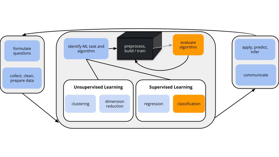
CONTEXT
world = supervised learning
We want to model some output variable \(y\) using a set of potential predictors (\(x_1, x_2, ..., x_p\)).
task = CLASSIFICATION
\(y\) is categorical and binary
(parametric) algorithm
logistic regression
application = classification
GOAL
\[\begin{split} \text{overall accuracy} & = \text{probability of making a correct classification} \\ \text{sensitivity} & = \text{true positive rate}\\ & = \text{probability of correctly classifying $y=1$ as $y=1$} \\ \text{specificity} & = \text{true negative rate} \\ & = \text{probability of correctly classifying $y=0$ as $y=0$} \\ \text{1 - specificity} & = \text{false positive rate} \\ & = \text{probability of classifying $y=0$ as $y=1$} \\ \end{split}\]
. . .
In-sample estimation (how well our model classifies the same data points we used to build it)
| y = 0 | y = 1 | |
|---|---|---|
| classify as 0 | a | b |
| classify as 1 | c | d |
\[\begin{split} \text{overall accuracy} & = \frac{a + d}{a + b + c + d}\\ \text{sensitivity} & = \frac{d}{b + d} \\ \text{specificity} & = \frac{a}{a + c} \\ \end{split}\]
. . .
k-Fold Cross-Validation (how well our model classifies NEW data points)
ROC: Receiver Operating Characteristic curves
. . .
Sensitivity and specificity depend upon the specific probability threshold c.
. . .
To understand this trade-off, for a range of possible thresholds c between 0 and 1, ROC curves calculate and plot
. . .
Why we care:
Open the QMD template for today.
Suppose we model RainTomorrow in Sydney using only the number of hours of bright Sunshine today.
Using a probability threshold of 0.5, this model produces the following classification rule:
Sunshine < 3.125, predict rain.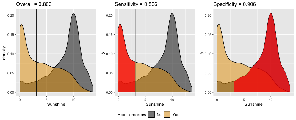
Interpret these in-sample estimates of the resulting classification quality.
Confirm the 3 metrics above using the confusion matrix. Work is shown below (peek when you’re ready).
            Truth
Prediction   No  Yes
       No  3108  588
Yes 324 602# Overall accuracy
(3108 + 602) / (3108 + 602 + 324 + 588)[1] 0.8026828# Sensitivity
602 / (602 + 588)[1] 0.5058824# Specificity
3108 / (3108 + 324)[1] 0.9055944We can change up the probability threshold in our classification rule!
The ROC curve for our logistic regression model of RainTomorrow by Sunshine plots the sensitivity (true positive rate) vs 1 - specificity (false positive rate) corresponding to “every” possible threshold:
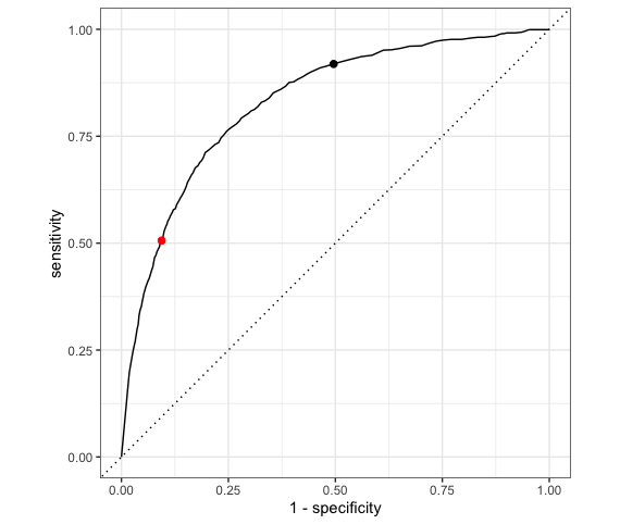
Which point represents the quality of our classification rule using a 0.5 probability threshold?
The other point corresponds to a different classification rule which uses a different threshold. Is that threshold smaller or bigger than 0.5?
Which classification rule do you prefer?
The area under an ROC curve (AUC) estimates the probability that our algorithm is more likely to classify y = 1 (rain) as 1 (rain) than to classify y = 0 (no rain) as 1 (rain), hence distinguish between the 2 classes.
AUC is helpful for evaluating and comparing the overall quality of classification models. Consider 3 different possible predictors (A, B, C) of rainy and non-rainy days:
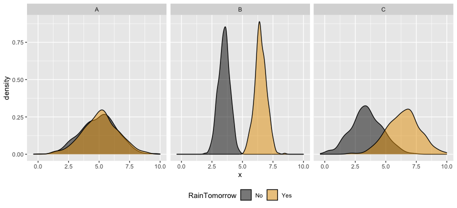
Which predictor is the “strongest” predictor of rain tomorrow?
. . .
The ROC curves corresponding to the models RainTomorrow ~ A, RainTomorrow ~ B, RainTomorrow ~ C are shown below.
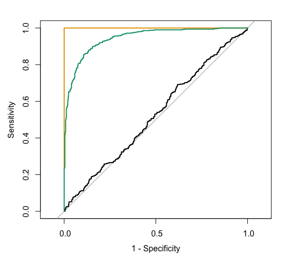
For each ROC curve, indicate the corresponding model and the approximate AUC. Do this in any order you want!
black ROC curve
RainTomorrow ~ ___green ROC curve
RainTomorrow ~ ___orange ROC curve
RainTomorrow ~ ___black ROC curve
RainTomorrow ~ Agreen ROC curve
RainTomorrow ~ Corange ROC curve
RainTomorrow ~ BIn general:
Today’s in-class exercises will be due as HW4.
Please find the exercises and template on Moodle.
I recommend working on Exercises 1, 5, and 6 in class.
Exercise 1 is necessary to the other exercises, and Exercises 5 and 6 involve new content: ROC curves, AUC, and LASSO for classification!
rpart and rpart.plot
Let my_model be a logistic regression model of categorical response variable y using predictors x1 and x2 in our sample_data.