8 KNN Regression and the Bias-Variance Tradeoff

Settling In

Sit with your Group Assignment 1 group
- Set up a communication venue (Slack channel, google chat, etc.) for your group to talk about Group Assignment 1 outside of class time
Prepare to take notes (find today’s QMD template on the Schedule page as usual!)
- Install the shiny and kknn packages if you haven’t already
Check Slack for any recent messages you may have missed

Preparing for Quiz 1

Logistics

When:

Wednesday, March 4, in class
first hour of class (not the whole 90 mins!)

Topics:

machine learning overview (Unit 0) and regression (Units 1–3)
both concepts and code
use the Course Learning Goals as a study guide!
code-related questions will focus on common patterns / functions that we’ve used a lot

Format:

on paper (no computers!)
closed notes (except for an instructor-provided R notesheet)
mix of multiple choice, fill-in-the-blank, short answer (1–2 sentences), and longer answer (1–2 paragraphs)
code-related questions will ask you to:
- fill-in-the-blank with the name of a function (eg set_mode) or argument (eg "regression")
- tell me what a line of code is doing (eg what does the step_dummy() function do?)
- tell me why we need a particular line of code (eg why do we need to use the step_dummy() function?)
- interpret output from a code chunk

Study Resources

HW3 (due Friday, Feb 27):

review the Important Notes before you begin!
designed to help you start studying for Quiz 1

Group Assignment 1 (due Friday, Mar 6):

designed to help you synthesize and practice the concepts from Units 0–3 and prepare for Quiz 1
we’ll have one day of in-class work time before the quiz (Mar 2), as well as 30 min right after the quiz (Mar 4)
until then, you should be working on this outside of class time (up to you to coordinate with your group!)
suggestion: complete steps 1–6 (see GA1 Instructions > Process) before our first in-class work day

Other resources (use, on your own, however you find useful):

Learning Goals

Clearly describe / implement by hand the KNN algorithm for making a regression prediction
Explain how the number of neighbors relates to the bias-variance tradeoff
Explain the difference between parametric and nonparametric methods
Explain how the curse of dimensionality relates to the performance of KNN

Notes: K Nearest Neighbors (KNN)

Context

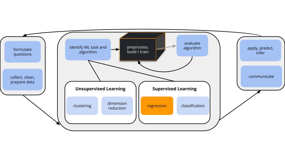
world = supervised learning
We want to model some output variable $y$ using a set of potential predictors ($x_1, x_2, ..., x_p$).
task = regression
$y$ is quantitative
(nonparametric) algorithm = K Nearest Neighbors (KNN)

Goal

Our usual parametric models (eg: linear regression) are too rigid to represent the relationship between $y$ and our predictors $x$. Thus we need more flexible nonparametric models.

KNN Regression

Goal
Build a flexible regression model of a quantitative outcome $y$ by a set of predictors $x$,
\[y = f(x) + \varepsilon\]

. . .

Idea
Predict $y$ using the data on “neighboring” observations. Since the neighbors have similar $x$ values, they likely have similar $y$ values.

. . .

Algorithm
For tuning parameter K, take the following steps to estimate $f(x)$ at each set of possible predictor values $x$:

Identify the K nearest neighbors of $x$ with respect to Euclidean distance.
Observe the $y$ values of these neighbors.
Estimate $f(x)$ by the average $y$ value among the nearest neighbors.

. . .

Output
KNN does not produce a nice formula for $\hat{f}(x)$, but rather a set of rules for how to calculate $\hat{f}(x)$.

. . .

In pictures (from ISLR)

Small Group Discussion

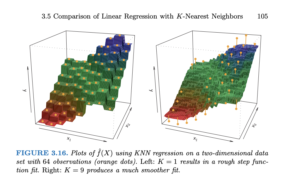
Discuss the following questions with your group.

Example 1: Review

Let’s review the KNN algorithm using a shiny app. Run the code below and ignore the syntax!!

Click “Go!” one time only to collect a set of sample data.
Check out the KNN with K = 1.
- What does it mean to pick K = 1?
- Where are the jumps made?
- Can we write the estimated $f(x)$ (red line) as $\beta_0 + \beta_1 x + ....$?
Now try the KNN with K = 25.
- What does it mean to pick K = 25?
- Is this more or less wiggly / flexible than when K = 1?
Set K = 100 where 100 is the number of data points. Is this what you expected?

Code

# Load packages and data
library(shiny)
library(tidyverse)
library(tidymodels)
library(kknn)
library(ISLR)

data(College)
college_demo <- College %>% 
  mutate(school = rownames(College)) %>% 
  filter(Grad.Rate <= 100)

Code

# Define a KNN plotting function
plot_knn <- function(k, plot_data){
  expend_seq <- sort(c(plot_data$Expend, seq(3000, 57000, length = 5000)))
  #knn_mod <- knn.reg(train = plot_data$Expend, test = data.frame(expend_seq), y = plot_data$Grad.Rate, k = k)
  knn_results <- nearest_neighbor() %>%
    set_mode("regression") %>% 
    set_engine(engine = "kknn") %>% 
    set_args(neighbors = k) %>% 
    fit(Grad.Rate ~ Expend, data = plot_data) %>% 
    augment(new_data = data.frame(Expend = expend_seq)) %>% 
    rename(expend_seq = Expend, pred_2 = .pred)
  ggplot(plot_data, aes(x = Expend, y = Grad.Rate)) + 
    geom_point() + 
    geom_line(data = knn_results, aes(x = expend_seq, y = pred_2), color = "red") + 
    labs(title = paste("K = ", k), y = "Graduation Rate", x = "Per student expenditure ($)") +
    lims(y = c(0,100))
}


# BUILD THE SERVER
# These are instructions for building the app - what plot to make, what quantities to calculate, etc
server_KNN <- function(input, output) {
  new_data <- eventReactive(input$do, {
    sample_n(college_demo, size = 100)
  })
  output$knnpic <- renderPlot({
    plot_knn(k = input$kTune, plot_data = new_data())
  })
}


# BUILD THE USER INTERFACE (UI)
# The UI controls the layout, appearance, and widgets (eg: slide bars).
ui_KNN <- fluidPage(
  sidebarLayout(
    sidebarPanel(
      h4("Sample 100 schools:"), 
      actionButton("do", "Go!"),
      h4("Tune the KNN algorithm:"), 
      sliderInput("kTune", "K", min = 1, max = 100, value = 1)
    ),
    mainPanel(
      h4("KNN Plot:"), 
      plotOutput("knnpic")
    )
  )
)


# RUN THE SHINY APP!
shinyApp(ui = ui_KNN, server = server_KNN)

KNN Details: Weighted Average

The tidymodels KNN algorithm predicts $y$ using weighted averages. The idea is to give more weight or influence to closer neighbors, and less weight to “far away” neighbors.

More details in the kknn package documentation.

Optional math:

Let ($y_1, y_2, ..., y_K$) be the $y$ outcomes of the K neighbors and ($w_1, w_2, ..., w_K$) denote the corresponding weights. These weights are defined by a “kernel function” which ensures that: (1) the $w_i$ add up to 1; and (2) the closer the neighbor $i$, the greater its $w_i$. Then the neighborhood prediction of $y$ is:

\[\sum_{i=1}^K w_i y_i\] The kernel wikipedia page shows common kernel functions.

The default “optimal” kernel used in kknn was defined in a 2012 Annals of Statistics paper.

Example 2: Bias-Variance Tradeoff

What would happen if we had gotten a different sample of data?!?

Bias: On average, across different datasets, how close are the estimates of $f(x)$ to the observed $y$ outcomes?
- We have high bias if our estimates are far from the observed $y$ outcomes
- We have low bias if our estimates are close to the observed $y$ outcomes
Variance: How variable are the estimates of $f(x)$ from dataset to dataset? Are the estimates stable or do they vary a lot?
- We have high variance if our estimates change a lot from dataset to dataset
- We have low variance if our estimates don’t change much from dataset to dataset

To explore the properties of overly flexible models, set K = 1 and click “Go!” several times to change the sample data. How would you describe how KNN behaves from dataset to dataset:
- low bias, low variance
- low bias, high variance
- moderate bias, low variance
- high bias, low variance
- high bias, high variance
To explore the properties of overly rigid models, repeat part a for K = 100:
- low bias, low variance
- low bias, high variance
- moderate bias, low variance
- high bias, low variance
- high bias, high variance
To explore the properties of more “balanced” models, repeat part a for K = 25:
- low bias, low variance
- low bias, high variance
- moderate bias, low variance
- high bias, low variance
- high bias, high variance

Example 3: Bias-Variance Reflection

In general…

Why is “high bias” bad?
Why is “high variability” bad?
What is meant by the bias-variance tradeoff?

Example 4: Bias-Variance Tradeoff for Past Algorithms

The LASSO algorithm depends upon tuning parameter $\lambda$:
- When $\lambda$ is too small, the model might keep too many predictors, hence be overfit.
- When $\lambda$ is too big, the model might kick out too many predictors, hence be too simple.
With this in mind:

For which values of $\lambda$ (small or large) will LASSO be the most biased?
For which values of $\lambda$ (small or large) will LASSO be the most variable?

The bias-variance tradeoff also comes into play when comparing across algorithms, not just within algorithms. Consider LASSO vs least squares:
- Which will tend to be more biased?
- Which will tend to be more variable?
- When will LASSO beat least squares in the bias-variance tradeoff game?

Exercises

Instructions

Work together. Collaboration improves higher-level thinking, confidence, communication, community, & more. Some tips:
- periodically check in with each other: see what exercise everyone is on, compare your answers, talk through the wording of any interpretation-related questions, see what questions people have
- when you have a question, ask your group before you ask me
- get to know each other as humans

Be kind to yourself (and each other). You will make mistakes! That’s part of the learning process.
Stay engaged. Studies show that when you’re working on an assignment for another class, continuously on your message app, playing games, etc. it impacts both your learning and the learning of those around you.

Questions

Context

Using the College dataset from the ISLR package, we’ll explore the KNN model of college graduation rates (Grad.Rate) by:

instructional expenditures per student (Expend)
number of first year students (Enroll)
whether the college is Private

# Load packages
library(tidymodels)
library(tidyverse)
library(ISLR)

# Load data
data(College)

# Wrangle the data
college_sub <- College %>% 
  mutate(school = rownames(College)) %>% 
  arrange(factor(school, levels = c("Macalester College", "Luther College", "University of Minnesota Twin Cities"))) %>% 
  filter(Grad.Rate <= 100) %>% 
  filter((Grad.Rate > 50 | Expend < 40000)) %>% 
  select(Grad.Rate, Expend, Enroll, Private)

Check out a codebook from the console:

?College

Goals

Understand how “neighborhoods” are defined using multiple predictors (both quantitative and categorical) and how data pre-processing steps are critical to this definition.
Tune and build a KNN model in R.
Apply the KNN model.
It is easier to review code than to deepen your understanding of new concepts outside class. Prioritize and focus on the concepts over the R code. You will later come back and reflect on the code.

Part 1: Identifying neighborhoods

The KNN model for Grad.Rate will hinge upon the neighborhoods defined by the 3 Expend, Enroll, and Private predictors. And these neighborhoods hinge upon how we pre-process our predictors.

We’ll explore these ideas below using the results of the following chunk. Run this, but DON’T spend time examining the code!

recipe_fun <- function(recipe){
  recipe <- recipe %>% 
    prep() %>% 
    bake(new_data = college_sub) %>% 
    head(3) %>% 
    select(-Grad.Rate) %>% 
    as.data.frame()
  row.names(recipe) <- c("Mac","Luther", "UMN")
  return(recipe)
}
# Recipe 1: create dummies, but don't standardize
recipe_1 <- recipe(Grad.Rate ~ Expend + Enroll + Private, data = college_sub) %>% 
  step_nzv(all_predictors()) %>% 
  step_dummy(all_nominal_predictors())
recipe_1_data <- recipe_fun(recipe_1)

# Recipe 2: standardize, then create dummies
recipe_2 <- recipe(Grad.Rate ~ Expend + Enroll + Private, data = college_sub) %>% 
  step_nzv(all_predictors()) %>% 
  step_normalize(all_numeric_predictors()) %>% 
  step_dummy(all_nominal_predictors())
recipe_2_data <- recipe_fun(recipe_2)

# Recipe 3: create dummies, then standardize
recipe_3 <- recipe(Grad.Rate ~ Expend + Enroll + Private, data = college_sub) %>% 
  step_nzv(all_predictors()) %>% 
  step_dummy(all_nominal_predictors()) %>%
  step_normalize(all_numeric_predictors())
recipe_3_data <- recipe_fun(recipe_3)

Feature space

Check out the feature space of our 3 predictors and take note of which school is the closer neighbor of Mac: UMN or Luther.

ggplot(college_sub, aes(x = Expend, y = Enroll, color = Private)) + 
  geom_point(alpha = 0.5) + 
  geom_text(data = head(college_sub, 3), aes(x = Expend, y = Enroll, label = c("Mac","Luther", "UMN")), color = "black")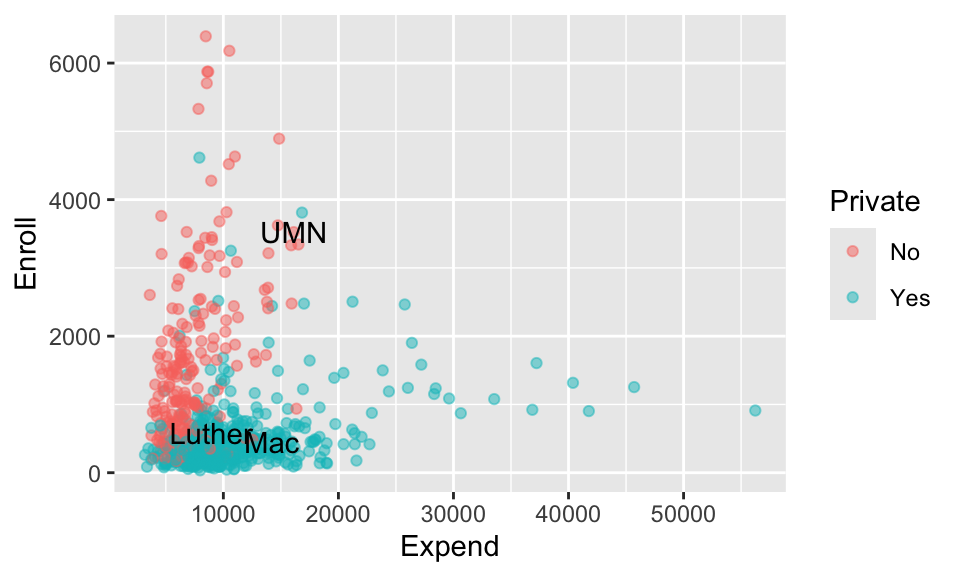

What happens when we don’t standardize the predictors?

Of course, KNN relies upon mathematical metrics (Euclidean distance), not visuals, to define neighborhoods. And these neighborhoods depend upon how we pre-process our predictors. Consider the pre-processing recipe_1 which uses step_dummy() but not step_normalize():

recipe_1_data

       Expend Enroll Private_Yes
Mac     14213    452           1
Luther   8949    587           1
UMN     16122   3524           0

Use this pre-processed data to calculate the Euclidean distance between Mac and Luther:

sqrt((14213 - ___)^2 + (452 - ___)^2 + (1 - ___)^2)

Check your distance calculation, and calculate the distances between the other school pairs, using dist().

dist(recipe_1_data)

By this metric, is Mac closer to Luther or UMN? So is this a reasonable metric? If not, why did this happen?

What happens when we standardize then create dummy predictors?
The metric above was misleading because it treated enrollments (people) and expenditures ($) as if they were on the same scale. In contrast, recipe_2 first uses step_normalize() and then step_dummy() to pre-process the predictors:

recipe_2_data

           Expend     Enroll Private_Yes
Mac     0.9025248 -0.3536904           1
Luther -0.1318021 -0.2085505           1
UMN     1.2776255  2.9490477           0

Calculate the distance between each pair of schools using these pre-processed data:

dist(recipe_2_data)

By this metric, is Mac closer to Luther or UMN? So is this a reasonable metric?

What happens when we create dummy predictors then standardize?
Whereas recipe_2 first uses step_normalize() and then step_dummy() to pre-process the predictors, recipe_3 first uses step_dummy() and then step_normalize():

recipe_3_data

           Expend     Enroll Private_Yes
Mac     0.9025248 -0.3536904   0.6132441
Luther -0.1318021 -0.2085505   0.6132441
UMN     1.2776255  2.9490477  -1.6285680

How do the pre-processed data from recipe_3 compare those to recipe_2?
RECALL: The standardized dummy variables lose some contextual meaning. But, in general, negative values correspond to 0s (not that category), positive values correspond to 1s (in that category), and the further a value is from zero, the less common that category is.
Calculate the distance between each pair of schools using these pre-processed data. By this metric, is Mac closer to Luther or UMN?

dist(recipe_3_data)

How do the distances resulting from recipe_3 compare to those from recipe_2?

dist(recipe_2_data)

Unlike recipe_2, recipe_3 considered the fact that private schools are relatively more common in this dataset, making the public UMN a bit more unique. Why might this be advantageous when defining neighborhoods? Thus why will we typically first use step_dummy() before step_normalize()?

college_sub %>% 
  count(Private)

Part 2: Build the KNN

With a grip on neighborhoods, let’s now build a KNN model for Grad.Rate.

For the purposes of this activity (focusing on concepts over R code), simply run each chunk and note what object it’s storing.

You will later be asked to come back and comment on the code.

STEP 1: Specifying the KNN model

knn_spec <- nearest_neighbor() %>%
  set_mode("regression") %>% 
  set_engine(engine = "kknn") %>% 
  set_args(neighbors = tune())

STEP 2: Variable recipe (with pre-processing)

Note that we use step_dummy() before step_normalize().

variable_recipe <- recipe(Grad.Rate ~ ., data = college_sub) %>% 
  step_nzv(all_predictors()) %>% 
  step_dummy(all_nominal_predictors()) %>%
  step_normalize(all_numeric_predictors())

STEP 3: workflow specification (model + recipe)

knn_workflow <- workflow() %>% 
  add_model(knn_spec) %>% 
  add_recipe(variable_recipe)

STEP 4: estimate multiple KNN models

This code builds 50 KNN models of Grad.Rate, using 50 possible values of K ranging from 1 to 200 (roughly 25% of the sample size of 775).

It then evaluates these models with respect to their 10-fold CV MAE.

set.seed(253)
knn_models <- knn_workflow %>% 
  tune_grid(
    grid = grid_regular(neighbors(range = c(1, 200)), levels = 50),
    resamples = vfold_cv(college_sub, v = 10),
    metrics = metric_set(mae)
  )

Part 3: Finalize and apply the KNN

Compare the KNN models
Plot the CV MAE for each of the KNN models with different tuning parameters K. NOTE: This is the same function we used for the LASSO!

knn_models %>% 
  autoplot()

Use this plot to describe the goldilocks problem in tuning the KNN:
- When K is too small, CV MAE increases because the model is too …
- When K is too big, CV MAE increases because the model is too …
Why did we try a range of K values?
In KNN modeling, we typically want to minimize the prediction errors. Given this goal, is the range of K values we tried wide enough? Or might there be a better value for K outside this range?
In KNN modeling, why won’t we typically worry about “parsimony”?

Pick K

Identify which value of K minimizes the CV MAE. Make sure this matches up with what you observe in the plot.

best_k <- knn_models %>% 
  select_best(metric = "mae")
best_k

Calculate and interpret the CV MAE for this model.

# Plug in a number or best_k$neighbors
knn_models %>% 
  collect_metrics() %>% 
  filter(neighbors == ___)

Final KNN model

Build your “final” KNN model using the optimal value you found for K above. NOTE: We only looked at roughly every 4th possible value of K (K = 1, 5, 9, etc). If we wanted to be very thorough, we could re-run our algorithm using each value of K close to our optimal K.

final_knn <- knn_workflow %>% 
  finalize_workflow(parameters = best_k) %>% 
  fit(data = college_sub)

What does a tidy() summary of final_knn give you? Does this surprise you?

# DO NOT REMOVE eval = FALSE
final_knn %>% 
  tidy()

Make some predictions
Check out Mac and Luther. NOTE: This is old data. Mac’s current graduation rate is one of the highest (roughly 90%)!

# Check out Mac & Luther
mac_luther <- college_sub %>% 
  head(2)
mac_luther

                   Grad.Rate Expend Enroll Private
Macalester College        77  14213    452     Yes
Luther College            77   8949    587     Yes

Use your KNN model to predict Mac and Luther’s graduation rates. How close are these to the truth?

# Prediction
___ %>% 
  ___(new_data = ___)

Do you have any idea why Mac’s KNN prediction is higher than Luther’s? If so, are you using context or something you learned from the KNN?

KNN pros and cons

What assumptions did the KNN model make about the relationship of Grad.Rate with Expend, Enroll, and Private?
What did the KNN model tell us about the relationship of Grad.Rate with Expend, Enroll, and Private?
Reflecting upon a and b, name one pro of using a nonparametric algorithm like the KNN instead of a parametric algorithm like least squares or LASSO.
Similarly, name one con.
Consider another “con”. Just as with parametric models, we could add more and more predictors to our KNN model. However, the KNN algorithm is known to suffer from the curse of dimensionality. Why? (A quick Google search might help.)

Parametric or nonparametric

Suppose we wanted to model the relationship of room and board costs vs out-of-state tuition. Would you use the parametric least squares algorithm or the nonparametric KNN algorithm?

ggplot(College, aes(x = Outstate, y = Room.Board)) + 
  geom_point()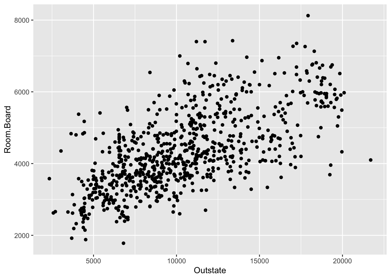

In general, in what situations would you use least squares instead of KNN? Why?

R code reflection

Revisit all code in Parts 2 and 3 of the exercises. Comment upon each chunk:

What is it doing?
How, if at all, does it differ from the least squares and LASSO code?

Varying our analysis: tuning parameter choice

We previously used select_best() to choose the number of neighbors $k$ that resulted in the lowest CV MAE.

Recall from our LASSO activity that we can also use select_by_one_std_err() to choose most simple model that produces a CV MAE that’s within 1 standard error of the best model (thus is not significantly worse). Review the code below:

# get "parsimonous" lambda
parsimonious_penalty <- lasso_models %>% 
  select_by_one_std_err(metric = "mae", desc(penalty))

Let’s figure out how to adapt this to the KNN setting.

Enter ?select_by_one_std_err in the Console to pull up the help page for this function.

Scroll down to the Arguments section, and note what the ... argument does.
Use select_by_one_std_err() to store the parsimonious choice for $k$ as parsimonious_k (or simple_k). (Our tuning parameter is called neighbors in tidymodels.)
Use knn_models %>% collect_metrics() %>% filter(neighbors == ___) to compare the CV MAE for the best $k$ to the $k$ for the simpler model.

Data drill

Calculate the mean Enroll for public vs private schools.

Plot the relationship of Grad.Rate vs Enroll, Private, and Expend.

Identify the private schools with first year enrollments exceeding 3000.

Ask and answer another question of interest to you.

Notes: R Code

Suppose we want to build a model of response variable y using predictors x1 and x2 in our sample_data.

# Load packages
library(tidymodels)
library(kknn)

Build the model

# STEP 1: KNN model specification
knn_spec <- nearest_neighbor() %>%
  set_mode("regression") %>% 
  set_engine(engine = "kknn") %>% 
  set_args(neighbors = tune())

STEP 1 notes:

We use the kknn, not lm, engine to build the KNN model.
The knn engine requires us to specify an argument (set_args):
- neighbors = tune() indicates that we don’t (yet) know an appropriate value for the number of neighbors $K$. We need to tune it.
By default, neighbors are defined using Euclidean distance. We could but won’t change this in the set_args().

# STEP 2: variable recipe
# (You can add more pre-processing steps.)
variable_recipe <- recipe(y ~ x1 + x2, data = sample_data) %>% 
  step_nzv(all_predictors()) %>% 
  step_dummy(all_nominal_predictors()) %>% 
  step_normalize(all_numeric_predictors())

# STEP 3: workflow specification (model + recipe)
knn_workflow <- workflow() %>% 
  add_recipe(variable_recipe) %>% 
  add_model(knn_spec)

# STEP 4: Estimate multiple KNN models using a range of possible K values
# Calculate the CV MAE & R^2 for each
set.seed(___)
knn_models <- knn_workflow %>% 
  tune_grid(
    grid = grid_regular(neighbors(range = c(___, ___)), levels = ___),
    resamples = vfold_cv(sample_data, v = ___),
    metrics = metric_set(mae, rsq)
  )

STEP 4 notes:

Since the CV process is random, we need to set.seed(___).
We use tune_grid() instead of fit() since we have to build multiple KNN models, each using a different tuning parameter K.
grid specifies the values of tuning parameter K that we want to try.
- the range specifies the lowest and highest numbers we want to try for K (e.g. range = c(1, 10). The lowest this can be is 1 and the highest this can be is the size of the smallest CV training set.
- levels is the number of K values to try in that range, thus how many KNN models to build.
resamples and metrics indicate that we want to calculate a CV MAE for each KNN model.

Tuning K

# Calculate CV MAE for each KNN model
knn_models %>% 
  collect_metrics()

# Plot CV MAE (y-axis) for the KNN model from each K (x-axis)
autoplot(knn_models)

# Identify K which produced the lowest ("best") CV MAE
best_K <- select_best(knn_models, metric = "mae")
best_K

# Get the CV MAE for KNN when using best_K
knn_models %>% 
  collect_metrics() %>% 
  filter(neighbors == best_K$neighbors)

Finalizing the “best” KNN model

# parameters = final K value (best_K or whatever other value you might want)
final_knn_model <- knn_workflow %>% 
  finalize_workflow(parameters = ___) %>% 
  fit(data = sample_data)

Use the KNN to make predictions

# Put in a data.frame object with x1 and x2 values (at minimum)
final_knn_model %>% 
  predict(new_data = ___)

Solutions

Small Group Discussion

Review

Solution

done
KNN with K = 1:
- predict grad rate using the data on the 1 closest neighbor
- where the neighorhood changes (in between observed points)
- no
KNN with K = 25:
- predict grad rate by average grad rate among 25 closest neighbors
- less wiggly / less flexible
probably not. it’s not a straight line. You might have expected a horizontal line at one value. There is a bit more going on to the algorithm (a weighted average).

Bias-Variance Tradeoff

Solution

low bias, high variance
high bias, low variance
moderate bias, low variance

Bias-Variance Reflection

Solution

On average, our prediction errors are large or high
The model is not stable / trustworthy, changes depending on the sample data
Ideally, both bias and variance would be low. BUT when we improve one of the features, we hurt the other.

Bias-Variance Tradeoff for Past Algorithms

Solution

.
- large. too simple / rigid
- small. too overfit / flexible
.
- LASSO. it’s simpler
- least squares. it’s more flexible
- when the least squares is overfit

Exercises

Part 1: Identifying neighborhoods

Feature space

Solution

Luther

What happens when we don’t standardize the predictors?

Solution

# a
sqrt((14213 - 8949)^2 + (452 - 587)^2 + (1 - 1)^2)

[1] 5265.731

# b
dist(recipe_1_data)

            Mac   Luther
Luther 5265.731         
UMN    3616.831 7750.993

UMN. The quantitative predictors are on different scales

What happens when we standardize then create dummy predictors?

Solution

Luther. Yes.

recipe_2_data

           Expend     Enroll Private_Yes
Mac     0.9025248 -0.3536904           1
Luther -0.1318021 -0.2085505           1
UMN     1.2776255  2.9490477           0

dist(recipe_2_data)

            Mac   Luther
Luther 1.044461         
UMN    3.471135 3.599571

What happens when we create dummy predictors then standardize?

Solution

recipe_3_data

           Expend     Enroll Private_Yes
Mac     0.9025248 -0.3536904   0.6132441
Luther -0.1318021 -0.2085505   0.6132441
UMN     1.2776255  2.9490477  -1.6285680

Private_Yes is now 0.6132441 or -1.6285680, not 1 or 0.
Luther

dist(recipe_3_data)

            Mac   Luther
Luther 1.044461         
UMN    4.009302 4.120999

The distance between Mac and Luther is the same, but the distance between Mac and UMN is bigger.

dist(recipe_2_data)

            Mac   Luther
Luther 1.044461         
UMN    3.471135 3.599571

Since public schools are more “rare”, the difference between Mac (private) and UMN (public) is conceptually bigger than if private and public schools were equally common.

Part 2: Build the KNN

Solution

No “answers” here. Just run the provided code and make note of what it’s doing.

STEP 1: Specifying the KNN model

knn_spec <- nearest_neighbor() %>%
  set_mode("regression") %>% 
  set_engine(engine = "kknn") %>% 
  set_args(neighbors = tune())

STEP 2: Variable recipe (with pre-processing)

Note that we use step_dummy() before step_normalize().

variable_recipe <- recipe(Grad.Rate ~ ., data = college_sub) %>% 
  step_nzv(all_predictors()) %>% 
  step_dummy(all_nominal_predictors()) %>%
  step_normalize(all_numeric_predictors())

STEP 3: workflow specification (model + recipe)

knn_workflow <- workflow() %>% 
  add_model(knn_spec) %>% 
  add_recipe(variable_recipe)

STEP 4: estimate multiple KNN models

This code builds 50 KNN models of Grad.Rate, using 50 possible values of K ranging from 1 to 200 (roughly 25% of the sample size of 775).

It then evaluates these models with respect to their 10-fold CV MAE.

set.seed(253)
knn_models <- knn_workflow %>% 
  tune_grid(
    grid = grid_regular(neighbors(range = c(1, 200)), levels = 50),
    resamples = vfold_cv(college_sub, v = 10),
    metrics = metric_set(mae)
  )

Part 3: Finalize and apply the KNN

Compare the KNN models

Solution

knn_models %>% 
  autoplot()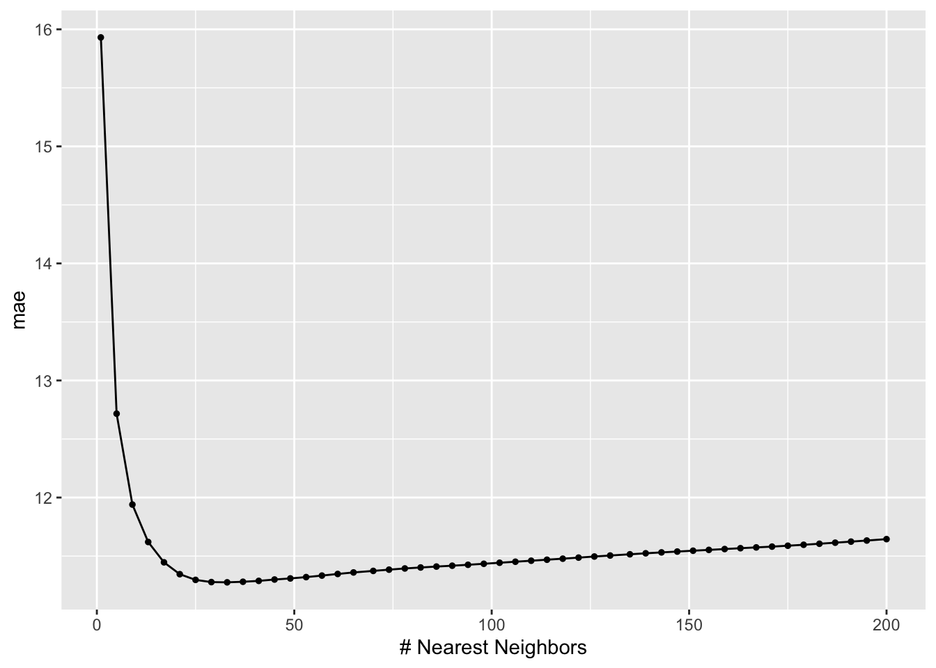

When K is too small, CV MAE increases because the model is too flexible (overfit). When K is too big, CV MAE increases because the model is too rigid (simple).
Because we can’t know in advance what a good value of K is.
Yes, it’s wide enough. We observe that CV MAE is minimized when K is around 25, it then increases from there.
KNN always uses all of the predictors we give it. The concept of parsimony in the sense of simplicity/complexity of how many variables are included is not relevant here. Changing $K$ does not lead to a simpler/more complex model in the way changing $\lambda$ does for LASSO.

Pick K

Solution

33 neighbors

best_k <- knn_models %>% 
  select_best(metric = "mae")
best_k

# A tibble: 1 × 2
  neighbors .config              
      <int> <chr>                
1        33 Preprocessor1_Model09

We expect the predictions of grad rate for new schools (not in our sample) to be off by 11.3 percentage points.

# Plug in a number
knn_models %>% 
  collect_metrics() %>% 
  filter(neighbors == 33)

# A tibble: 1 × 7
  neighbors .metric .estimator  mean     n std_err .config              
      <int> <chr>   <chr>      <dbl> <int>   <dbl> <chr>                
1        33 mae     standard    11.3    10   0.516 Preprocessor1_Model09

# an equivalent but more reproducible way to do this:
knn_models %>% 
  collect_metrics() %>% 
  filter(neighbors == best_k$neighbors)

# A tibble: 1 × 7
  neighbors .metric .estimator  mean     n std_err .config              
      <int> <chr>   <chr>      <dbl> <int>   <dbl> <chr>                
1        33 mae     standard    11.3    10   0.516 Preprocessor1_Model09

Final KNN model

Solution

final_knn <- knn_workflow %>% 
  finalize_workflow(parameters = best_k) %>% 
  fit(data = college_sub)

Since this is a nonparametric method, we can’t summarize the functional relationship between our outcome and predictors with parameters and thus tidy() doesn’t have estimates to give us.

Make some predictions

Solution

# Prediction
mac_luther <- college_sub %>% 
  head(2)

final_knn %>% 
  predict(new_data = mac_luther)

# A tibble: 2 × 1
  .pred
  <dbl>
1  78.8
2  75.7

If you have any ideas, it’s probably based on context because the KNN hasn’t given us any info about why it returns higher or lower predictions of grad rate.

KNN pros and cons

Solution

essentially none – just that colleges with similar expenditures, enrollments, and school types (private vs public) would have similar graduation rates
not much – we can just use it for predictions
KNN doesn’t make assumptions about relationships (which is very flexible!)
KNN doesn’t provide much insight into the relationships between y and x
When calculated by more and more predictors, our nearest neighbors might actually be far away (thus not very similar).

Parametric or nonparametric

Solution

least squares. the relationship is linear, so doesn’t require the flexibility of a nonparametric algorithm
when the relationships of interest can be reasonably represented by least squares, we should use least squares. It provides much more insight into the relationships.

R code reflection

Solution

Come to office hours to discuss.

Varying our analysis: tuning parameter choice

Solution

The help page tells us that select_by_one_std_err() sorts the models from most simple to most complex. For a tuning parameter p, we use:

ml_models %>% select_by_one_std_err(metric = "mae", p) (if smaller values of p indicate a simpler model)
ml_models %>% select_by_one_std_err(metric = "mae", desc(p)) (if larger values of p indicate a simpler model)

So for KNN we want:

simple_k <- select_by_one_std_err(knn_models, metric = "mae", desc(neighbors))

knn_models %>%
  collect_metrics() %>%
  filter(neighbors==simple_k$neighbors)

# To show CV results for both simple_k and best_k
knn_models %>%
  collect_metrics() %>%
  filter(neighbors==c(best_k$neighbors, simple_k$neighbors))

Follow-up questions to consider:

What does “parsimony” or “simplicity” mean in the context of a KNN model? How does this differ from the LASSO context?
If you are fitting a KNN model in the future, which select_ function would you use, and why?

Data drill

Solution

# a
college_sub %>% 
  group_by(Private) %>% 
  summarize(mean(Enroll))

# A tibble: 2 × 2
  Private `mean(Enroll)`
  <fct>            <dbl>
1 No               1641.
2 Yes               457.

# b
ggplot(college_sub, aes(y = Grad.Rate, x = Enroll, size = Expend, color = Private)) + 
  geom_point(alpha = 0.5)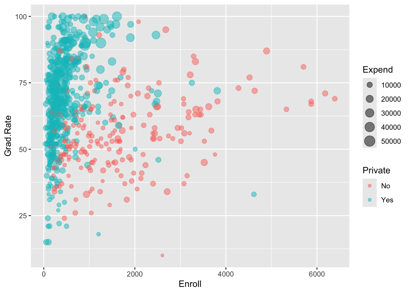

# c
college_sub %>% 
  filter(Enroll > 3000, Private == "Yes")

                                  Grad.Rate Expend Enroll Private
Boston University                        72  16836   3810     Yes
Brigham Young University at Provo        33   7916   4615     Yes
University of Delaware                   75  10650   3252     Yes

Answers will vary. Come to office hours to discuss.

Wrapping Up

Today’s Material

Wrap up the activity, check the solutions, and check out the optional resources posted for today.
Remember that there’s an R code reference section at the bottom of these notes!

Upcoming Deadlines

CP7: due before our next class
HW3: due Feb 27
- Note the different structure and instructions for this HW (please read carefully before you begin!)
- Designed to help you start studying for Quiz 1
GA1: due Mar 6
- Get started now! See suggestions above about which steps to complete before our in-class work day on Mar 2.
- This is great practice / review of code & concepts
Quiz 1: in class on Mar 4