# load packages
library(tidymodels)
library(tidyverse)

# STEP 1: specify a linear regression model
lm_spec <- linear_reg() %>%
  set_mode("regression") %>%
  set_engine("lm")

# STEP 2: variable recipe
# Add a pre-processing step that does PCA on the predictors
# num_comp is the number of PCs to keep (we need to tune it!)
# remove the update_role line if you don't have an ID variable you want to ignore in your model/PCA
pcr_recipe <- recipe(y ~ ., data = sample_data) %>%
  update_role(data_id, new_role = "id") %>%
  step_dummy(all_nominal_predictors()) %>%
  step_normalize(all_predictors()) %>%
  step_pca(all_predictors(), num_comp = tune())

# STEP 3: workflow
pcr_workflow <- workflow() %>%
  add_recipe(pcr_recipe) %>%
  add_model(lm_spec)

# STEP 4: Estimate multiple PCR models trying out different numbers of PCs to keep
# For the range, the biggest number you can try is the number of predictors you started with
# Put the same number in levels
set.seed(___)
pcr_models <- pcr_workflow %>%
  tune_grid(
    grid = grid_regular(num_comp(range = c(1, ___)), levels = ___),
    resamples = vfold_cv(sample_data, v = 10),
    metrics = metric_set(mae)
)20 Principal Component Regression
Unsupervised & supervised learning are friends!
Settling In
- Sit with your NEW group and introduce yourselves
- Prepare to take notes
- Catch up on any announcements you’ve missed on Slack
- FYI: revised OH time on Friday! (8:30–9:30 am)
Announcements
Quiz 3 is coming up soon!
Date: during our final exam block
Format: same as Quizzes 1 and 2
Content: cumulative, but at least half will focus on unsupervised learning (concepts + code)
- Study Tips:
- Create a study guide using the “Learning Goals” page on the course website
- Fill out the STAT 253 Concepts Maps (slides 9–11)
- Work on Group Assignment 3
- Review old CPs, HWs, and in-class exercises
- Come to office hours with questions!
Learning Goals
- Explain the goal of dimension reduction and how this can be useful in a supervised learning setting
- Clearly describe / implement the principal component regression algorithm
- Describe the tradeoff of choice of principal components (\(k\)) in terms of the bias-variance tradeoff
- Implement strategies for choosing \(k\)
- Discuss the pros and cons of principal component regression relative to variable selection and LASSO
Small Group Discussion
Let’s review some ideas from last class!
Example 1
What is the goal of Principal Component Analysis?
Example 2
Consider the following PCA results from a paper written by Macalester faculty (Sarah Boyer, Biology; Dennis Cao, Chemistry) and student collaborators:
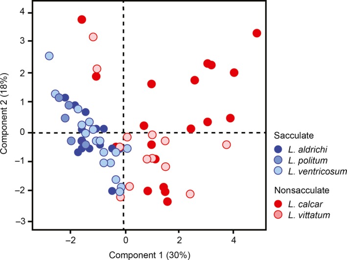
What is this type of plot called?
If the authors want to retain at least 50% of the variance in the original features, how many/which PCs should they keep?
When describing this figure in their paper, the authors say: “Principal components analysis (PCA) on the free amino acid profiles of the harvestmen specimens yielded four PCs with eigenvalues exceeding 1, which collectively explain 70.6% of the total variation in amino acid composition. PC1 explains 30.2% of the variation and is characterized by positive loading of alanine, valine, phenylalanine, glutamic acid, and tyrosine, and negative loading of isoleucine and threonine. PC2 accounts for a further 17.7% of the variation and is characterized by positive loading of …”
- What is a loading?
- What is the connection between loadings and scores?
- What can we learn from loadings about the original features?
Bonus
Fun Fact: Professor Grinde’s latest paper is also about PCA (and PC Regression)!
Check it out here if you’re interested: Adjusting for principal components can induce collider bias in genome-wide association studies.
Notes: PC Regression
Context
We’ve been distinguishing 2 broad areas in machine learning:
- supervised learning: when we want to predict / classify some outcome y using predictors x
- unsupervised learning: when we don’t have any outcome variable y, only features x
- clustering: examine structure among the rows with respect to x
- dimension reduction: examine & combine structure among the columns x
BUT sometimes we can combine these ideas!
Combining Forces
Dimension Reduction + Clustering
Use dimension reduction to visualize / summarize lots of features and notice interesting groups.
Example: many physical characteristics of penguins, many characteristics of songs, etcUse clustering to identify interesting groups.
Example: types (species) of penguins, types (genres) of songs, etc
Clustering + Classification
Use clustering to identify interesting groups.
Example: types (species) of penguins, types (genres) of songs, etcThese groups might then become our \(y\) outcome variable in future analysis.
Example: classify new penguins as one of the “species” we identified, classify new songs as one of the “genres” we identified
EXAMPLE: K-means clustering + Classification of news articles
Dimension Reduction + Regression: Dealing with lots of predictors
Suppose we have an outcome variable \(y\) (quantitative OR categorical) and lots of potential predictors \(x_1, x_2, ..., x_p\). Perhaps we even have more predictors than data points (\(p > n\))!
This idea of measuring lots of things on a sample is common in genetics, image processing, video processing, or really any scenario where we can grab data on a bunch of different features at once. For simplicity, computational efficiency, avoiding overfitting, etc, it might benefit us to simplify our set of predictors.
There are a few approaches:
variable selection (eg: using backward stepwise)
Simply kick out some of the predictors.NOTE: This does not work when \(p > n\).
regularization (eg: using LASSO)
Shrink the coefficients toward / to 0.NOTE: This sorta works when \(p > n\).
feature extraction (eg: using PCA)
Identify & utilize only the most salient features of the original predictors. Specifically, combine the original, possibly correlated predictors into a smaller set of uncorrelated predictors which retain most of the original information.NOTE: This does work when \(p > n\).
Principal Component Regression (PCR)
Step 1
Ignore \(y\) for now. Use PCA to combine the \(p\) original, correlated predictors \(x\) into a set of \(p\) uncorrelated PCs.Step 2
Keep only the first \(k\) PCs which retain a “sufficient” amount of information from the original predictors.Step 3
Model \(y\) by these first \(k\) PCs.
PCR vs Partial Least Squares
When combining the original predictors \(x\) into a smaller set of PCs, PCA ignores \(y\). Thus PCA might not produce the strongest possible predictors of \(y\).
Partial least squares provides an alternative.
Like PCA, it combines the original predictors into a smaller set of uncorrelated features, but considers which predictors are most associated with \(y\) in the process.
Chapter 6.3.2 in ISLR provides an optional overview.
Small Group Discussion
Example 3
For each scenario below, indicate which would (typically) be preferable in modeling y by a large set of predictors x: (1) PCR; or (2) variable selection or regularization.
- We have more potential predictors than data points (\(p > n\)).
- It’s important to understand the specific relationships between y and x.
- The x are NOT very correlated.
Exercises
Use the rest of class time to work on HW7
Exercises 3 focuses on PC Regression. In Exercise 4, you will compare your PC Regression model to LASSO. Use the R Code Notes below to help with this!
Remember to set.seed(253) on any exercises that involve randomness.
Notes: R Code
Suppose we have a set of sample_data with multiple predictors x, a quantitative outcome y, and (possibly) a column named data_id which labels each data point. We could adjust this code if y were categorical.
RUN THE PCR algorithm
FOLLOW-UP
Processing and applying the results is the same as for our other tidymodels algorithms!
Review previous notes to remind yourself how functions like autoplot, select_by_one_std_err, and collect_metrics work.
Wrapping Up
- As usual, take time after class to finish any remaining exercises, check solutions, reflect on key concepts from today, and come to office hours with questions
- Upcoming due dates:
- Group Assignment 3: review instructions before next class
- HW7 (last one!!): Apr 27
- Quiz 2 Revisions: Apr 29
- Learning Reflection 4: May 4
- Quiz 3: during our assigned final exam block
Solutions
Small Group Discussion
Example 1
Solution:
Combine the original, potentially correlated, features into a smaller number of uncorrelated columns.Solution:
score plot
more than two, although we can’t tell the exact number from this figure. all we can see is that the first two PCs collectively explain 48% of the variance. adding one or two more should do the trick, but we’d need to check our scree plot to be sure.
..
- loadings are coefficients/weights. they tell us how much each of the original variables contributes to the new features (PCs)
- the scores are constructed by multiplying the original feature values by their corresponding loadings
- from loadings, we can learn which features play the biggest role / contribute most substantially to each PC. we can also learn which of the original features are positively (or negatively) correlated with one another.
Example 3
Solution:
- (typically) can’t do variable selection, regularization when \(p > n\).
- The PCs lose the original meaning of the predictors
- PCR wouldn’t simplify things much (need a lot of PCs to retain info).
Exercises
Solutions:
Solutions will not be provided. These exercises are part of your homework this week.