library(tidyverse)library(tidymodels)library(rpart) # for building treeslibrary(rpart.plot) # for plotting treeslibrary(randomForest) # for bagging & forestslibrary(infer) # for resamplinglibrary(fivethirtyeight)data("candy_rankings")
# What are the 6 most popular candies?# The least popular?
Build an unpruned tree
For demonstration purposes only let’s:
define a popularity variable that categorizes the candies as “low”, “medium”, or “high” popularity
NOTE: Creating a categorical outcome variable will turn this into a classification problem. This is not strictly necessary here — trees can also be used for regression! You’ll explore this in HW5.
delete the original winpercent variable
rename variables to make them easier to read in a tree
Our goal is to model candy popularity by all possible predictors in our data.
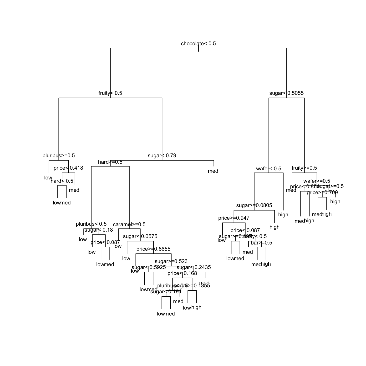
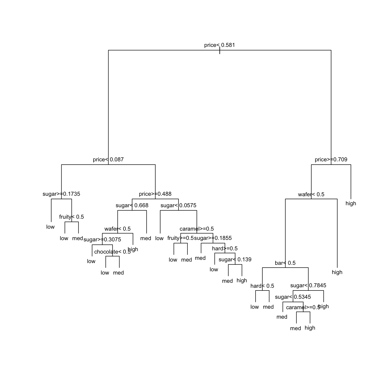
# STEP 1: tree specificationtree_spec <-decision_tree() %>%set_mode("classification") %>%set_engine(engine ="rpart") %>%set_args(cost_complexity =0, min_n =2, tree_depth =30)# STEP 2: Build the tree! No tuning (hence no workflows) necessary.original_tree <- tree_spec %>%fit(popularity ~ ., data = candy)# Plot the treeoriginal_tree %>%extract_fit_engine() %>%plot(margin =0) original_tree %>%extract_fit_engine() %>%text(cex =0.7)
Ideally, our classification algorithm would have both low bias and low variance:
low variance = the results wouldn’t change much if we changed up the data set
low bias = within any data set, the predictions of y tend to have low error / high accuracy
Unfortunately, like other overfit algorithms, unpruned trees don’t enjoy both of these. They have (SELECT ONE)…
low bias, low variance
low bias, high variance
high bias, low variance
high bias, high variance
New Concept
GOAL
Maintain the low bias of an unpruned tree while decreasing variance.
APPROACH
Build a bunch of unpruned trees from different data. This way, our final result isn’t overfit to our sample data.
THE RUB (CHALLENGE/DIFFICULTY)
We only have 1 set of data…
Take a REsample of candy
We only have 1 sample of data. But we can resample it (basically pretending we have a different sample).
Let’s each take our own unique candy resample (aka bootstrapping):
Take a sample of 85 candies from the original 85 candies, with replacement.
Some data points will be sampled multiple times while others aren’t sampled at all.
On average, 2/3 of the original data points will show up in the resample and 1/3 will be left out.
Take your resample:
# Set the seed to YOUR 7-digit phone number (skip the country and area codes)set.seed(1234567)# Take a REsample of candies from our samplemy_candy <-sample_n(candy, size =nrow(candy), replace =TRUE)# Check it outhead(my_candy, 3)dim(my_candy)
In the next exercise, we’ll each build a tree of popularity using our own resample data.
First, check your intuition:
TRUE / FALSE: All of our trees will be the same.
TRUE / FALSE: Our trees will use the same predictor (but possibly a different cut-off) in the first split.
TRUE / FALSE: Our trees will use the same predictors in all splits.
TipFun Math Facts
With resampling (also known as bootstrapping), we have an original sample of \(n\) rows. We drawn individual rows with replacement from this set until we have another set of size \(n\).
The probability of choosing any one row (say the 1st row) on the first draw is \(1/n\). The probability of not choosing that one row is \(1-1/n\). That is just for the first draw. There are \(n\) draws, all of which are independent, so the probability of never choosing this particular row on any of the draws is \((1-1/n)^n\).
If we consider larger and larger datasets (large \(n\) going to infinity), then
Thus, the probability that any one row is NOT chosen is about 1/3 and the probability that any one row is chosen is 2/3.
Build & share YOUR tree
Build and plot a tree using your unique sample (my_candy):
# Build your treemy_tree <- tree_spec %>%fit(popularity ~ ., data = my_candy)# Plot your treemy_tree %>%extract_fit_engine() %>%plot(margin =0) my_tree %>%extract_fit_engine() %>%text(cex =0.7)
Use your tree to classify Baby Ruth, the 7th candy in the original data.
Do this “by hand” first, using the tree you created above and info about the Baby Ruth predictor values:
candy[7,]
          chocolate fruity caramel nutty nougat wafer  hard  bar pluribus sugar
Baby Ruth      TRUE  FALSE    TRUE  TRUE   TRUE FALSE FALSE TRUE    FALSE 0.604
          price popularity
Baby Ruth 0.767        med
Then check your prediction using R code:
my_tree %>%predict(new_data = candy[7,])
Finally, share your results!
Record your prediction and paste a picture of your tree into this document.
Using our FOREST
We now have a group of multiple trees – a forest!
These trees…
differ from resample to resample
don’t use the same predictor in each split (not even in the first split)!
produce different popularity predictions for Baby Ruth
Based on our forest of trees (not just your 1 tree), what’s your prediction for Baby Ruth’s popularity?
What do you think are the advantages of predicting candy popularity using a forest instead of a single tree?
Can you anticipate any drawbacks of using forests instead of trees?
Notes: Bagging and Forests
BAGGING (Bootstrap AGGregatING) & Random Forests
To classify a categorical response variable y using a set of p predictors x:
Take B resamples from the original sample.
Sample WITH replacement
Sample size = original sample size n
Use each resample to build an unpruned tree.
For bagging: consider all p predictors in each split of each tree
For random forests: at each split in each tree, randomly select and consider only a subset of the predictors (often roughly p/2 or \(\sqrt{p}\))
Use each of the B trees to classify y at a set of predictor values x.
Average the classifications using a majority vote: classify y as the most common classification among the B trees.
Ensemble Methods
Bagging and random forest algorithms are ensemble methods.
They combine the outputs of multiple machine learning algorithms.
As a result, they decrease variability from sample to sample, hence provide more stable predictions / classifications than might be obtained by any algorithm alone.
Pros & Cons
Order trees, random forests, & bagging from least to most computationally expensive.
What results will be easier to interpret: trees or forests?
Which of bagging or random forests will produce a collection of trees that tend to look very similar to each other, and similar to the original tree? Hence which of these algorithms is more dependent on the sample data, thus will vary more if we change up the data? [both questions have the same answer]
Exercises
For the rest of the class, work together on Exercises 1–7
Tuning parameters (challenge)
Our random forest of popularity by all 11 possible predictors will depend upon 3 tuning parameters:
trees = the number of trees in the forest
mtry = number of predictors to randomly choose & consider at each split
min_n = minimum number of data points in any leaf node of any tree
Check your intuition.
Does increasing the number of trees make the forest algorithm more or less variable from dataset to dataset?
We have 11 possible predictors, and sqrt(11) is roughly 3. Recall: Would considering just 3 randomly chosen predictors in each split (instead of all 11) make the forest algorithm more or less variable from dataset to dataset?
Recall that using unpruned trees in our forest is important to maintaining low bias. Thus should min_n be small or big?
Build the forest
Given that forests are relatively computationally expensive, we’ll only build one forest using the following tuning parameters:
mtry = NULL: this sets mtry to the default, which is sqrt(number of predictors)
trees = 500
min_n = 2
Fill in the below code to run this forest algorithm.
# There's randomness behind the splits!set.seed(253)# STEP 1: Model Specificationrf_spec <-rand_forest() %>%set_mode("___") %>%___(engine ="ranger") %>%___(mtry =NULL,trees =500,min_n =2,probability =FALSE, # Report classifications, not probability calculationsimportance ="impurity"# Use Gini index to measure variable importance )# STEP 2: Build the forest# There are no preprocessing steps or tuning, hence no need for a workflow!candy_forest <- ___ %>%fit(___, ___)
Use the forest for prediction
Use the forest to predict the popularity level for Baby Ruth. (Remember that its real popularity is “med”.)
candy_forest %>%predict(new_data = candy[7,])
Evaluating forests: concepts
But how good is our forest at classifying candy popularity?
To this end, we could evaluate 3 types of forest predictions.
Why don’t in-sample predictions, i.e. asking how well our forest classifies our sample candies, give us an “honest” assessment of our forest’s performance?
Instead, suppose we used 10-fold cross-validation (CV) to estimate how well our forest classifies new candies. In this process, how many total trees would we need to construct?
Alternatively, we can estimate how well our forest classifies new candies using the out-of-bag (OOB) error rate. Since we only use a resample of data points to build any given tree in the forest, the “out-of-bag” data points that do not appear in a tree’s resample are natural test cases for that tree. The OOB error rate tracks the proportion or percent of these out-of-bag test cases that are misclassified by their tree. How many total trees would we need to construct to calculate the OOB error rate?
Moving forward, we’ll use OOB and not CV to evaluate forest performance. Why?
Evaluating forests: implementation
Report and interpret the estimated OOB prediction error.
candy_forest
The test or OOB confusion matrix provides more detail. Use this to confirm the OOB prediction error from part a. HINT: Remember to calculate error (1 - accuracy), not accuracy.
# NOTE: t() transposes the confusion matrix so that # the columns and rows are in the usual ordercandy_forest %>%extract_fit_engine() %>%pluck("confusion.matrix") %>%t()
Which level of candy popularity was least accurately classified by our forest?
Check out the in-sample confusion matrix. In general, are the in-sample predictions better or worse than the OOB predictions?
# The cbind() includes the original candy data# alongside their predicted popularity levelscandy_forest %>%predict(new_data = candy) %>%cbind(candy) %>%conf_mat(truth = popularity,estimate = .pred_class )
          Truth
Prediction low med high
      low   18   0    0
      med    6  39    2
      high   1   0   19
Variable importance
Variable importance metrics, averaged over all trees, measure the strength of the 11 predictors in classifying candy popularity:
# Print the metricscandy_forest %>%extract_fit_engine() %>%pluck("variable.importance") %>%sort(decreasing =TRUE)# Plot the metricslibrary(vip)candy_forest %>%vip(geom ="point", num_features =11)
If you’re a candy connoisseur, does this ranking make some contextual sense to you?
The only 2 quantitative predictors, sugar and price, have the highest importance metrics. This could simply be due to their quantitative structure: trees tend to favor predictors with lots of unique values. Explain. HINT: A tree’s binary splits are identified by considering every possible cut / split point in every possible predictor.
Classification regions
Just like any classification model, forests divide our data points into classification regions.
Let’s explore this idea using some simulated data that illustrate some important contrasts.1
Import and plot the data:
# Import datasimulated_data <-read.csv("https://mac-stat.github.io/data/circle_sim.csv") %>%mutate(class =as.factor(class))# Plot dataggplot(simulated_data, aes(y = X2, x = X1, color = class)) +geom_point() +theme_minimal()
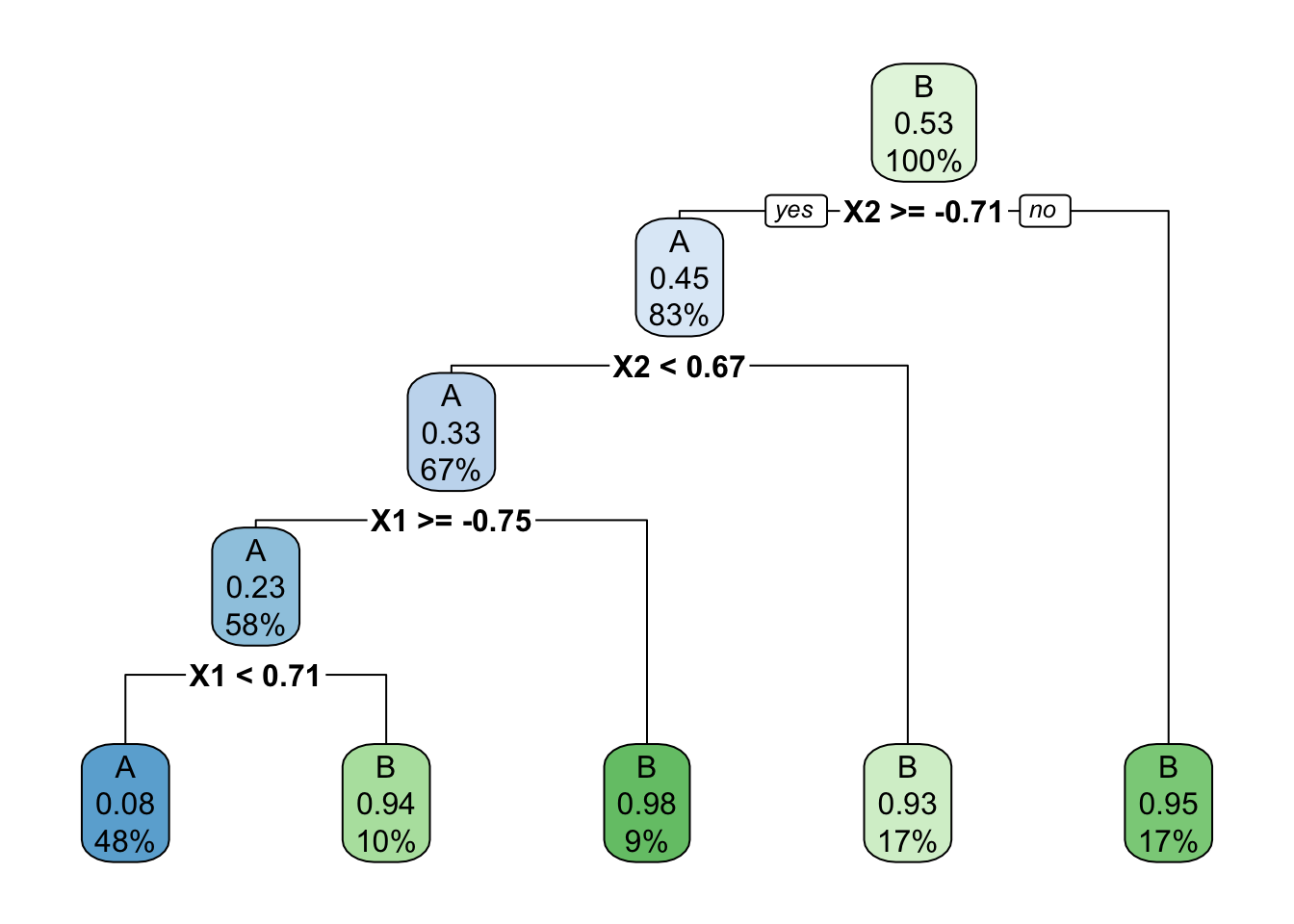
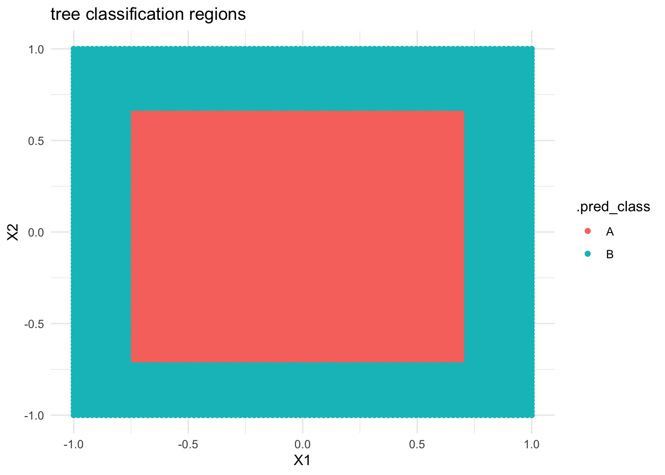
Below is a classification tree of class by X1 and X2. What do you think its classification regions will look like?
# Build the (default) treecircle_tree <-decision_tree() %>%set_mode("classification") %>%set_engine(engine ="rpart") %>%fit(class ~ ., data = simulated_data)circle_tree %>%extract_fit_engine() %>%rpart.plot()
Check your intuition. Were you right?
# THIS IS ONLY DEMO CODE.# Plot the tree classification regionsexamples <-data.frame(X1 =seq(-1, 1, len =100), X2 =seq(-1, 1, len =100)) %>%expand.grid()circle_tree %>%predict(new_data = examples) %>%cbind(examples) %>%ggplot(aes(y = X2, x = X1, color = .pred_class)) +geom_point() +labs(title ="tree classification regions") +theme_minimal()
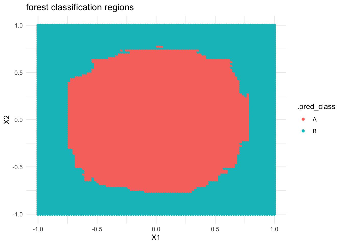
If we built a forest model of class by X1 and X2, what do you think the classification regions will look like?
Check your intuition. Were you right?
# THIS IS ONLY DEMO CODE.# Build the forestcircle_forest <- rf_spec %>%fit(class ~ ., data = simulated_data)# Plot the tree classification regionscircle_forest %>%predict(new_data = examples) %>%cbind(examples) %>%ggplot(aes(y = X2, x = X1, color = .pred_class)) +geom_point() +labs(title ="forest classification regions") +theme_minimal()
Reflect on what you’ve observed here!
If you finish early
Do one of the following:
Check out the optional “Deeper learning” section below on another ensemble method: boosting.
Check out group assignment 2 on Moodle. Next class, your group will pick what topic to explore.
Work on homework.
Deeper learning
Boosting
Extreme gradient boosting, or XGBoost, is yet another ensemble algorithm for regression and classification. We’ll consider the big picture here. If you want to dig deeper:
Section 8.2.3 of the book provides a more detailed background
Like bagging and forests, boosting combines predictions from B different trees.
BUT these trees aren’t built from B different resamples. Boosting trees are grown sequentially, each tree slowly learning from the previous trees in the sequence to improve in areas where the previous trees didn’t do well. Loosely speaking, data points with larger misclassification rates among previous trees are given more weight in building future trees.
Unlike in bagging and forests, trees with better performance are given more weight in making future classifications.
Bagging vs boosting
Bagging typically helps decrease variance, but not bias. Thus it is useful in scenarios where other algorithms are unstable and overfit to the sample data.
Boosting typically helps decrease bias, but not variance. Thus it is useful in scenarios where other algorithms are stable, but overly simple.
Notes: R code
Suppose we want to build a forest or bagging algorithm of some categorical response variable y using predictors x1 and x2 in our sample_data.
# Load packageslibrary(tidymodels)library(rpart)library(rpart.plot)# Resolves package conflicts by preferring tidymodels functionstidymodels_prefer()
We’ll typically use the following tuning parameters:
trees = 500 (the more trees we use, the less variable the forest)
min_n = 2 (the smaller we allow the leaf nodes to be, the less pruned, hence less biased our forest will be)
mtry
for forests: mtry = NULL (the default) will use the “floor”, or biggest integer below, sqrt(number of predictors)
for bagging: set mtry to the number of predictors
# STEP 1: Model Specificationrf_spec <-rand_forest() %>%set_mode("classification") %>%set_engine(engine ="ranger") %>%set_args(mtry = ___,trees =500,min_n =2,probability =FALSE, # give classifications, not probability calculationsimportance ="impurity"# use Gini index to measure variable importance )# STEP 2: Build the forest or bagging model# There are no preprocessing steps or tuning, hence no need for a workflow!ensemble_model <- rf_spec %>%fit(y ~ x1 + x2, data = sample_data)
Use the model to make predictions / classifications
# Put in a data.frame object with x1 and x2 values (at minimum)ensemble_model %>%predict(new_data = ___)
Examine variable importance
# Print the metricsensemble_model %>%extract_fit_engine() %>%pluck("variable.importance") %>%sort(decreasing =TRUE)# Plot the metrics# Plug in the number of top predictors you wish to plot# (The upper limit varies by application!)library(vip)ensemble_model %>%vip(geom ="point", num_features = ___)
My tree looks like this (yours will be a little different):
Code
# Take a REsample of candies from our sampleset.seed(1234567)my_candy <-sample_n(candy, size =nrow(candy), replace =TRUE)# Build your treemy_tree <- tree_spec %>%fit(popularity ~ ., data = my_candy)# Plot your treemy_tree %>%extract_fit_engine() %>%plot(margin =0) my_tree %>%extract_fit_engine() %>%text(cex =0.7)
Based on this tree, we predict Baby Ruth are medium popularity:
my_tree %>%predict(new_data = candy[7,])
# A tibble: 1 × 1
  .pred_class
  <fct>
1 med
Using our FORESTS
Solution:
take the majority vote, i.e. most common category
by averaging across multiple trees, classifications will be more stable / less variable from dataset to dataset (lower variance)
computational intensity (lack of efficiency), harder to visualize / interpret
Notes
pros & cons
Solution:
trees, forests, bagging
trees (we can’t draw a forest)
bagging (forests tend to have lower variability)
Exercises
Tuning parameters (challenge)
Solution:
less variable (less impacted by “unlucky” trees)
less variable
small
Build the forest
Solution:
# There's randomness behind the splits!set.seed(253)# STEP 1: Model Specificationrf_spec <-rand_forest() %>%set_mode("classification") %>%set_engine(engine ="ranger") %>%set_args(mtry =NULL,trees =500,min_n =2,probability =FALSE, # give classifications, not probability calculationsimportance ="impurity"# use Gini index to measure variable importance )# STEP 2: Build the forest# There are no preprocessing steps or tuning, hence no need for a workflow!candy_forest <- rf_spec %>%fit(popularity ~ ., data = candy)
Use the forest for prediction
Solution:
candy_forest %>%predict(new_data = candy[7,])
# A tibble: 1 × 1
  .pred_class
  <fct>
1 med
Evaluating forests: concepts
Solution:
they use the same data we used to build the forest
10 forests * 500 trees each = 5000 trees
1 forest * 500 trees = 500 trees
it’s much more computationally efficient
Evaluating forests: implementation
Solution:
We expect our forest to misclassify roughly 40% of new candies.
.
# APPROACH 1: # of MISclassifications / total # of classifications(6+1+15+6+2+4) / (8+29+14+6+1+15+6+2+4)
predictors with lots of unique values have far more possible split points to choose from
Classification regions
Solution:
…
# THIS IS ONLY DEMO CODE.# Plot the tree classification regionsexamples <-data.frame(X1 =seq(-1, 1, len =100), X2 =seq(-1, 1, len =100)) %>%expand.grid()circle_tree %>%predict(new_data = examples) %>%cbind(examples) %>%ggplot(aes(y = X2, x = X1, color = .pred_class)) +geom_point() +labs(title ="tree classification regions") +theme_minimal()
…
# THIS IS ONLY DEMO CODE.# Build the forestcircle_forest <- rf_spec %>%fit(class ~ ., data = simulated_data)# Plot the tree classification regionscircle_forest %>%predict(new_data = examples) %>%cbind(examples) %>%ggplot(aes(y = X2, x = X1, color = .pred_class)) +geom_point() +labs(title ="forest classification regions") +theme_minimal()
Forest classification regions are less rigid / boxy than tree classification regions.
Wrapping Up
As usual, take time after class to finish any remaining exercises, check solutions, reflect on key concepts from today, and come to office hours with questions